If sample size was a person, "actually...” would be its favorite word. Sample size turns otherwise interesting storylines into dry, statistical fact. Me: "That 12 game hit streak from a player means he's finally breaking out of his slump, right?" Sample Size: "No, you need 100 PA before drawing any relevant conclusions on hitting performance" Me: "Wow I can't wait to watch Jameson Taillon face off against Jackson Chourio tonight. Chourio really seems to have his number" Sample Size: "Chourio's success against Taillon is purely a product of chance. You should have no expectations that his performance against Taillon will continue".
Unfortunately, Sample Size is usually right. At least insofar as the number of data points we have access to is usually directly correlated to trust in the observed trend for any probabilistic process. Without an adequate sample size it's impossible to separate signal from noise. That said, I think there's some beauty in the noise that we observe before the signal emerges. The stochastic nature of baseball that creates pockets of hit streaks, postseason tears, batters that rake against specific pitchers etc. are part of what we all love about the sport. Even if many of them are product of chance made possible by small sample sizes, the narratives and story lines are ultimately valuable for their own stake. And the cool thing is every once in a while, one of these story lines turns out to not simply be a product of probability theory, but a legitimate trend. Unfortunately, baseball romanticism can't factor into the mindset of scouts, R&D teams, and the sports betting community whose baseball analysis becomes the constant art of separating signal from noise; More accurately, identifying that signal before your competitors.
But how can we know when the signal emerges? When can we confidently say that a hitter's .350 avg to start the season is sustainable (many people were asking this with Luis Arraez in 2023). How many games do I need to see before I can trust a player's performance? How big does the sample size need to be? Well this post is about tackling this problem systematically. Let's start with batters and define some specific questions. Namely, how many games do I need to see from a player before I can expect their On-Base + Slugging (OPS) to hold for the season? Does this vary much player to player?
Willson Contreras caught a lot of heat during the beginning of 2023. His new Cardinals team was losing and people wanted someone to blame. Contreras replacing HOFer and beloved Cardinal, Yadier Molina gave fans an easy target, leading to him becoming the de-facto scapegoat for the spiraling team. Now I'm a Cubs fan and as much as I relished in the newfound dysfunction of the Cardinals, I couldn't help but start to feel for the guy. It was obvious that the issues with the Cardinals ran much deeper than Contreras. But in some ways I get the Cardinals' frustration. Willson was brought in to add offense at the catcher position and he simply wasn't hitting. His OPS through the first two months of the year (March 30 - May 30) was 0.654. Not great. At the time, this was cause for panic from Cardinals fans. Two months is a large sample size right? It looked like something had happened to one of the league's top offensive catchers. Nope. Contreras ended up raising his OPS to 0.826 by the end of the season, a full 0.172 points. The takeaway? We jumped to a conclusion too early, driven by trying to fit limited information to a story that we wanted to be true before waiting for the requisite body of evidence to confirm it. Humans just cannot go without creating narratives. After all, the assertion "Contreras's 0.654 OPS is likely caused by some component of getting unlucky and random chance" isn't nearly as flashy as "Contreras is washed and can't handle the pressure of filling Molina's spot in St. Louis."
The interesting thing is that Contreras didn't even top the list of the largest differences between OPS through May and season OPS for players with at least 100 PAs. In fact, he was 14th. Michael Harris II started the season with a 0.534 OPS through two months and finished with 0.808. That's an incredible run. In the other direction Owen Miller started the season with a red-hot OPS of 0.871 and finished the season with a 0.674 OPS. I've outlined how these player stats can change drastically even from what you'd think would be a solid two-month sample size to end of the year. So that begs the question: At what point during the season can I trust a player's OPS, or any statistic for that matter? This is the question I will be attempting to answer in this post.
Starting with first principles let's define what causes noisy, untrustworthy stats: Variance. Sampling a statistic with a higher variance will require more samples to accurately estimate the mean, or the signal. So we'll start by saying that the standard deviation (the metric we'll use for variance) should be correlated in some way to the "stability", or "settling time" of a statistic.
What do I mean by “stability” and “settling time”? Simply put, how long (how many games) does it take for a stat to “even out”, or settle to a value that represents a player's true ability? There are many different ways to approach this question and therefore calculate stability as we've defined it. For this post, we are going to explore one such approach. What I'm choosing to call Sliding Window Stability. I may look at other methods eventually in a future follow-up post.
So how does it work? Well let's go back to back to our Standard Deviation variable. If we look at the current value of any given statistic as the season progresses, we expect that the sample standard deviation will continue to decrease and for the mean to progressively converge to the end value because our sample size, or N, continues to increase. This is pretty straightforward and perhaps even a bit obvious, but let's look at a specific example to really hammer home this idea. Below is a graphic of Ian Happ's OPS over the course of the 2024 season with the x-axis representing games played.
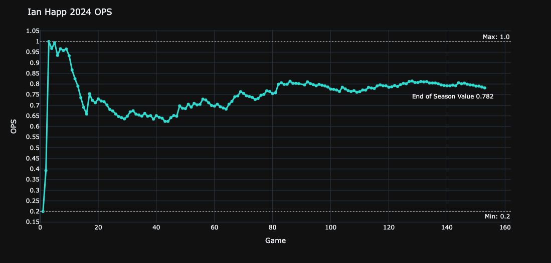
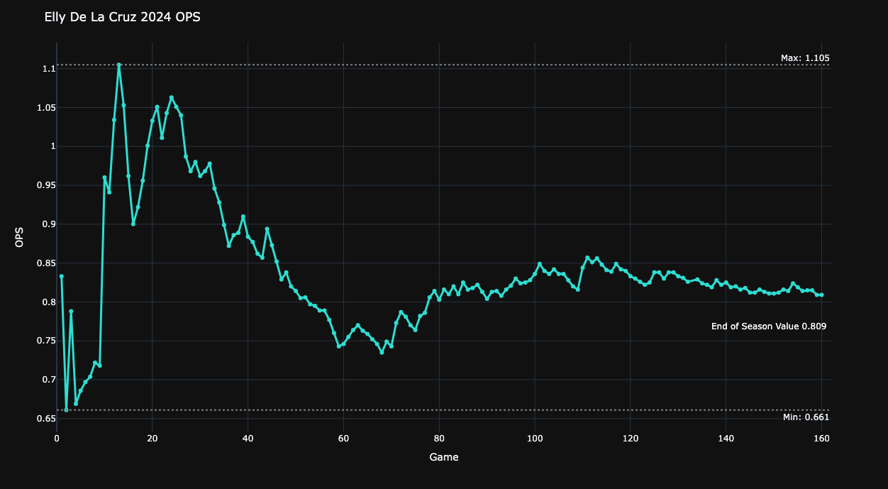
The settling phenomenon becomes immediately clear when we look at a chart like this. We see how as we accumulate more games into our sample size, the trajectory stabilizes. Here's another example:
It's pretty clear that there's a certain point where the stat becomes relatively close to the number that it will eventually finish as for the season. So how do we determine quantitatively where this point is? Well, one way to do this is to apply a threshold to some type of rolling window - let's say the standard deviation over the last 10 games played. Note, even though we're just looking at the latest 10 games in this case, we're still calculating the season standard deviation at each of those data points. As we progress through the season, the standard deviation of the season OPS over the latest 10 games will decrease and if we apply some type of threshold value, let's say 0.04, then we can find the exact game when our data smooths out to a point where we can say it's stable.
This is a good start, but it has some problems if used in isolation. First, obviously the size of the window and threshold we choose is going to have a huge impact on what we consider stable? How do we determine what the values of these should be? - let's put a pin in that for now. The second issue with just using standard deviation as a metric of stability is that temporary periods of perceived stability prior to actual stability are quite common in baseball. It's not uncommon over a 10 game stretch for a player to consistently get about 1 hit per game, resulting in little change to a season rolling statistic, such as OPS. Yet, they might follow this up with a 10 game cold streak, only logging a couple of hits over the entire period, resulting in a large impact to the season OPS. Therefore, I propose we look at another parameter, what we'll call Standard Deviation Rate of Change. My assertion is that it's not only important to look at the current standard deviation, but also how the standard deviation has changed recently, essentially a standard deviation velocity, or derivative parameter. I choose to calculate this by adding another trailing 10 game window behind our first window. We'll compare the difference between the current standard deviation and that of our trailing window. That way if we just went from a highly unstable period to a weirdly, or prematurely stable period, we don't mistake this for true stability. Essentially this eliminates false positives in our calculation, allowing us to avoid the illusion of stability before it actually occurs. Like our standard deviation approach, we can apply a threshold to the std dev ROC. Now we have two parameters, and we want both to be true before we say a stat has settled.
So, this is a great start for establishing statistical criteria for baseball stability, but I would argue we can go further. What's nice about our current approach is that it is a forward-looking metric, and we don't require any prior knowledge aside from the data that exists up until today to make a prediction of stability. However, I would argue that this isn't taking advantage of the fact that we have a lot of historical data to look back on and draw additional conclusions from. For instance, how long did it take Bryce Harper's OPS to settle in 2024, or every player in the league for that matter? We should take advantage of the entire picture of players' performances over the years to see when a stat really settled. For instance, one thing we can look at is how the season mean calculated through a given number of games compared to a player's ending season value. It's as simple as mean_diff = season_mean - current_mean. Again, we can apply a threshold here to determine the game when the mean was close to the ending mean. Of course, on its own, just using this metric for stability criteria has a lot of problems. It's likely that a player's current performance will bounce around their eventual season performance, producing periods of times where our criteria is satisfied, well before the statistic has settled. However, when we combine this with our other criteria, we begin to get a more comprehensive way to evaluate stability. Essentially, we can look back at historical player performances, go game by game, and calculate all of these metrics and apply our thresholds. Our criteria will look for all three metrics to cross our thresholds. When they do, we will say that the stat has stabilized for X player at Y games. We can then do this same process for each player that satisfied some number of Plate Appearances for the season, and average our results, creating a general estimate for needed games played for stability for each batting statistic mentioned earlier.
Here's a couple animations to show how this works. Let's look at Bryce Harper's OPS first:
Use the play/pause button to control the animation.
And here's one for Willi Castro:
Use the play/pause button to control the animation.
We can apply this same process to any player, giving us an automated way to try out different thresholding criteria. With the basic criteria I used to create those animations, it's noticible that Harper's OPS reaches our settling criteria 20 games before Castro's. But how do we choose those thresholds? Well, I admit this requires a bit of trial and error. My approach is through iteration of the aforementioned process. When we look at stability across all players for given stability criteria, that will inevitably result in variance in the resulting games_to_stability metric we derive at the end. Some players will reach their stability criteria faster than others. When we average across all players, we'll have a distribution of games_to_stability. We don't want this spread to be too large, otherwise that will imply our criteria is too loose. Too tight and we might be waiting longer than we need to to say a stat has stabilized. So I suggest we iterate our thresholds until we reach a desired macro-level spread of stability across all players. Here's where it gets a bit subjective.
When picking thresholds, as opposed to shooting randomly in the dark, we can orient ourselves by looking at the stability of the stability metrics themselves. If we have an idea of where the mean_diff gets small and where the standard deviation tends to settle, these will be good starting points for our selection of thresholds.
The relationship between the thresholds as a function of games played for all qualified hitters' 2024 OPS is shown below. To make use of all the data, we're limited to the minimum number of total games played by a player in our dataset which is why our charts don't include the full 162 regular season games. Additionally, we start these charts at 10 games as this is the first time we begin computing our rolling standard deviation. The std dev ROC compares two windows which requires at least 20 games.
It's pretty apparent that each statistic decays exponentially at first, before settling into either a linear delcine or constant value. For each chart, we can find the elbow where they transition out of their steep declines. I've plotted a reference line around where I think this happens. For the rolling mean, this is around 25 games, the standard deviation plot is about 30 games, and 35 games for the std dev ROC plot. Ok, so if nothing else gives us an idea for the order of magnitude of each of these settling thresholds and an idea of what values we can pick first.
So my approach will be to select a set of three values, one for each of our thresholds. We'll then iterate through every qualified player season in 2024, checking our threshold values against the computed value at each game played throughout the season. At some point, all of our criteria will be met and we'll log at which game this occured for that player. We'll then compile all of the results from each player season and compute the mean and standard deviation, representing league averages for these values. This will give us an overall "average games to stabilization" metric and the variation of said metric. Then we'll repeat this process for a new set of thresholds, and again until we have around 10 or so tests completed. If we were being rigorous, we would use a grid search or some other method to sweep over a continuous range of input threshold values. Instead, we hand selected a set of 10 which limits our ability to optimize this problem. I'd rather this post serve as an exploration into this problem rather than a research paper so for now, we'll just leave it here.
Here are the results shown next to our chosen thresholds:
We want low numbers for all of our settling statistics. Fewer Mean Games-to-Stablity means we're able to reach our predictive thresholds quickly and predict season outcomes earlier in a season. A small standard deviation of this same statistic means it's a reliable stabilization point and doesn't vary much player to player. And a low "Avg OPS Error" means that at the predicted stabilization point (say 50 games), the difference between a player's OPS at that point and their OPS at the end of the season is small. So ideally, we're looking to accurately predict season-end OPS as early as possible. I've color coded the results for readability - relatively low values are green with larger values red. We're looking for a set of thresholding criteria that results in greens across the board. Unfortunately, as you would expect this isn't really possible. To get a more accurate OPS prediction, we'd want tight stability criteria which requires more games in our sample size (i.e., larger Mean Games-to-Stability). Conversly, an early prediction often results in higher OPS error. The best we can hope for is a compromise.
Requiring a small Delta Mean (the difference between the predicted value and final value) shrinks our OPS error the most, as we would expect, however this usually coincides with longer Games-to-Stability. Even the smallest of OPS errors that we're able to achieve are still relatively large in this case. Take the second test case: Here we are able to get within 39 points of the final OPS after 64.4 regular season games, about 1/3 of the way through the season, albeit with a large standard deviation. This is pretty good, but I think even at this point we're only able to say that OPS is "starting to stabilize". It turns out that in baseball even a sample size of 64 games is small and likely too early to draw conclusions from.
There's a couple ways we could improve this exploration in the future. First, as I mentioned earlier, we should employ a more rigorous method for selecting our input thresholds, potentially using something like a grid search to find an optimal set of thresholds and truly answer our question of when OPS stabilizes. Our 10-game and 20-game windows for computing standard deviation and ROC respectively was somewhat arbitrary. We should try different window sizes. Lastly, we only looked at OPS in this post. We should see how settling trends change for other stats like OBP, K%, etc.
It turns out there are many ways to measure the stability of baseball statistics, and while this post looked at a relatively simple method using the idea of statistical thresholds and a sliding game window, we're only scratching the surface. I hope to revisit this topic again in the future and expand on what we did here. For now, the most sure conclusion we can draw is that whether we like it or not, sample size matters.