Fine Wine or Milk? Part 1: The WAR/G Aging Curve

Baseball researchers such as Jeff Zimmerman and Mitchel Lichtman have written extensively on aging curves. In his 2011 article Hitter Aging Curves and 2013 follow-up, Are Aging Curves Changing?, Zimmerman introduced aging curves as a way to model the trajectory of players' skill over time. He found that historically, wRC+ increased early in a player's career before peaking around age 26, and then declining. In fact, most aging curves, whether they are based on wRC+, OPS, or some other offensive metric, generally have a similar shape:

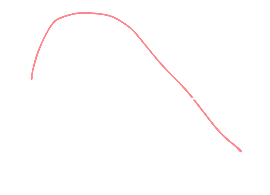
There's been hints that the aging curve may be changing though. Coinciding with the end of the PED era, Zimmerman concluded that players no longer showed the same early-career growth. Instead of peaking around age 26, as earlier studies indicated, recent performance seemed to rise more gradually, and peak earlier. The era-dependency of aging curves is just one aspect of their complexity, and the depth of the problem has kept researchers coming back to it, seeking to develop a generalized model that holds across contexts. After all, knowing when a player is likely to peak or decline has enormous implications for front offices.

Zimmerman's study of how a value-focused stat like RAA ages provides a basis for our work. While his focus was on era-to-era differences, I'll look at how WAR's components age relative to one another, using his methods as a starting point. One aspect that I have found to be underwhelming and the area that we'll look to expand on is the modeling of multiple variables in the aging curve. In this first post of a two-parter, we'll derive a WAR/G aging curve that is not only a function of age, but also skill.

Let's start by looking at the existing modeling approaches. To create his RAA aging curve, Zimmerman used an approach called the "Delta method," introduced by Mitchel Lichtman, which compares players' consecutive-season stats, aggregates a weighted mean of all players over a given time span, and then models performance as a function of age. While effective, this method is not bulletproof. It requires our dataset to have players with consecutive seasons, which consequently filters out players who did not play or meet the qualifying threshold in the following season. As Mitchel Lichtman pointed out in 2016, this introduces a bias: "lucky" players who overperform their true skill are more likely to return the following year than "unlucky" underperformers, skewing curves toward sharper declines. The natural regression to the mean from the overperformers in this case is incorrectly interpreted as an aging effect.

Lichtman later proposed corrections, but these introduce complexity while still requiring us to throw out non-consecutive player seasons, a data processing step that removes a significant amount of data from our dataset.
Ideally, we would use a more robust method. Enter the Generalized Additive Model (GAM): instead of relying on seasonal pairs, the GAM method uses thin plate regression to fit a spline to performance as a function of age while controlling for each player's career average. This allows the inclusion of all seasonal pairs while reducing survivorship bias.

Jonathan Judge compared performance of the GAM vs the Delta and Delta Corrected methods and showed that the GAM outperformed both in terms of fitting past data (1977-2016) and in predicting held-out careers. Although more research will assuredly result in even more improved methods for age curve modeling, as of today the GAM stands out as our most reliable tool.

In practice, regardless of method, these models were used to collapse all player trajectories into a single, universal aging curve by effectively averaging across all seasons in the dataset. This provides a useful, but limited insight - it tells us the average expected WAR/G by age. However, this averaging obscures the fact that aging curves vary with ability - the path of a superstar is not the same as that of a replacement-level player. What we really need is a way to model aging as a function of both age and ability. Conveniently, the GAM allows us to model multiple variables.

My goal in this article is not to recreate the work of others or come up with yet another way to model aging curves for individual stats. Between Zimmerman, Lichtman, Judge, and others, those models have been well-studied and parametrized. Instead, I want to refine how we model player value as a function of age, extending existing univariate approaches that create a universal aging curve to bivariate models that depend on both age and ability.

We'll use WAR as a proxy for value in our analysis, and start by creating the univariate, average WAR-based aging curve. Then we'll incorporate a term in our model to account for baseline ability level, allowing the aging curve to change shape based on a player's skill.

The first step is computing season-average WAR/game for each qualifying player season between 2005 and 2024. We then fit a GAM spline to the resulting data. Our 2005-2024 period omits years in the 90s and 00s when many players were taking substances that could...skew...performance. But beyond just eliminating steroid seasons, this narrower range is likely more indicative of current aging trends based on modern physical conditioning and recovery science. As we already discussed, the aging curve has changed based on era, but I want to remove this effect for this study. The tradeoff is that we only use a sample of 19 years, which we should keep in mind when interpreting results. It is also worth mentioning that there have been other attempts to fit parametric regression models to aging data, such as JC Bradbury's quadratic approach, however, his model required fitting a symmetrical quadratic to the aging curve, which doesn't account for different rates of improvement and decline.

For each year between 2005 and 2024, I grouped each position player by age, divided WAR by games, and included that player's career mean WAR/G. This leaves us with something like the following for a given player season:

When creating our model, even the univariate model, we need to control for survivorship bias: only the most elite players debut young and stick around into their late 30s. These are the players that are going to be the most unaffected by age. Without correcting for this, we would observe an effect where aging effects in the mid to late 30s appear much tamer than they actually are, resulting in an artificially shallow or stable aging curve. For our univariate model, we'll use a very simple correction method, while the bivariate model will account for this in the model itself by adding ability level as a term in the equation. For both methods we use a GAM regression approach to compute our aging curve. For the univariate model, we correct for survivorship bias by baselining each player's WAR/G for a given season against their own career WAR/G average, effectively anchoring each player to their own baseline and producing a "WAR/G above career average" metric for each player season. This centers each player's performance around their own career average before fitting. When we apply the GAM to these data points, we are effectively modeling the average trajectory of being above/below one's own career norm. Our GAM equation in this case is quite straightforward because there is only one nonlinear component that we're fitting.

Computing the GAM for our univariate model and correcting for survivorship bias via a centering method produces the following chart:

This chart shows the averaged WAR/G aging curve across all qualified player seasons from 2005 to 2024. Each faint dot represents a player season, the data points that our model uses to fit the spline. I included these to show the density of our dataset. As the chart indicates, the sample is sparse at the youngest and oldest ages, with most players clustered between 25 and 31. Consistent with expectations, players increase their value until peaking around age 26, after which their season-over-season WAR/G begins to decline, typically starting around age 30.

But this approach lacks an important nuance: skill and aging are connected. Think about it - elite players aren't just great because they have a higher peak; they also tend to defy typical patterns of age-related decline. Accordingly, we should treat the WAR/G aging curve not as static but as dynamic with its shape changing as a function of a player's baseline skill level. Rather than simply subtracting a player's career average to normalize across ability, we should instead fold that average directly into the GAM as a covariate. When we do so, our equation becomes:

By incorporating each player's career avg WAR/G as a covariate, the model learns distinct aging trajectories based on player skill. Shown here are examples for a 0.032 Career WAR/G player (95th percentile), 0.023 Career WAR/G player (75th percentile), a 0.016 WAR/G player (50th percentile), a 0.010 career WAR/G player (25th percentile), and a 0.004 career WAR/G player (5th percentile). For the 50th percentile player, the curve looks very similar to our univariate, average-player model. You'll notice, however, that the shape of our trajectories change slightly as we deviate from this mean-ability level. More skilled players (above the 50th percentile) peak later and sustain their peak longer than below average skill players. This finding coincides with our intuition - aging curves vary by player skill.

So we've found that a player's aging curve is dependent not only on age, but also ability. But we can go even further. How players provide value is not the same. WAR is comprised of Batting, Baserunning, and Fielding runs, and two players with equal WAR may achieve it very differently. The next question I want to answer is which of them maintains value longer? We'll get into this in part 2 of this series. Stay tuned!